Boxplots with Jitter

Boxplots are a good way to examine the distribution of data. They allow you to see outliers and understand how it skews.

The image below comes from the the US Labor Department 2011 Time Use Survey.

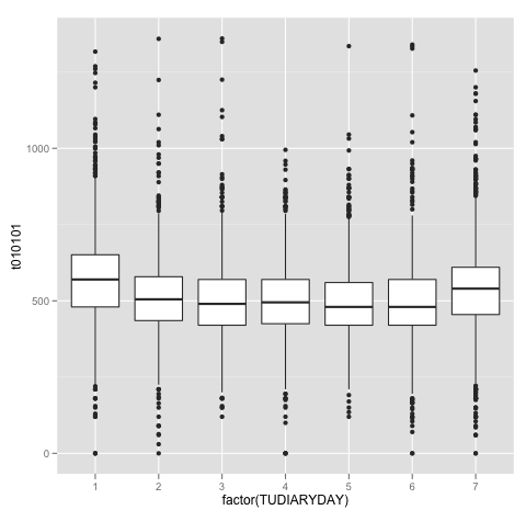
The X-axis represents days of the week, Sunday = 1 and Saturday = 7. Along the Y-axis is t010101, the variable for ‘time sleeping’, and it is expressed in the form of minutes. This is what I see when I first crack open some data. It’s raw.

You see a box and you see a dark line inside that box. The dark line is the MEDIAN, and the box contains half of all the observations in the sample. the dots represent individuals at the far ends. (John Tukey introduced the boxplot visual in 1977.)

Jitter

The simplest term for Jitter that I know is ‘random’. Jitter can be thought of as a random dispersal.

The issue with the box plot with dots is that dots overlap. It’s a problem I wrote about on Scatterplots back in late May. You can solve that problem with Hexagonal Binning (Hexbin). But not in boxplots. The answer is to apply Jitter to sort them all out.

Check out the plot below using library(ggplot2):
 

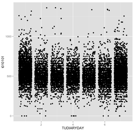
The jitter scatters out the series so you get a good sense of what’s going on. In the previous chart, you may have believed that only 1 person on a Sunday reported 0 hours of sleep. In the chart above, you can see that’s it 3. The smearing of the records horizontally is applied randomly. There is no horizontal meaning within a day.

Density

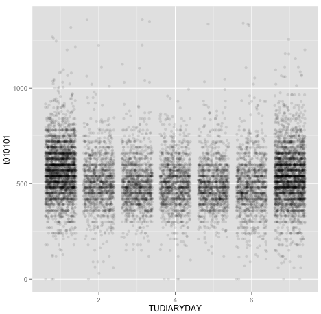
There are some 12,479 individual dots you’re looking at. Since everything is getting an equal weight, it’s hard to see intensity. This can be addressed using the translucency variable ALPHA. You can see the result below.

Do you notice how much darker the weekends are compared to the weekdays? That’s the visible manifestation of those two days getting oversampled.

I ran gender (Male = 1, Female = 2) through the same variable, and got the visual below:

And finally, I can combine Gender, Day Of The Week, and Sleep together into a single treatment:

Light Blue are Females, Dark Blue are Males – and you can see the distributions.

So what are the charts telling me? Americans are sleeping in on Saturday and Sunday… so stop the presses. You could tell, from the first boxplot, that the medians were higher.


In Sum

• You can use boxplots to see variation in data

• You can use jitter to reveal details that weren’t obvious

• You can use color to expand your story

 PS (
 
And:

There’s considerable effort involved in cleaning up the raw visuals and converting them into presentation-ready formats. It’s a very mundane point in analytics today, but worth covering off here. If you’re trying to do a persuasive post about sleeping-in dynamics, it’s important to have all those labels on. Some readers may be interested to know that our software(s) doesn’t produce professional grade visualizations on their own(!).

Tasks I neglected:

• A proper title for each chart

• Labeling the axis titles

• Labeling the axis variables

• Getting the color variation gradient reduced to just two colors

• Recoding the Y-Axis to hours instead of minutes

• Applying proper color frame

)

***

I’m Christopher Berry.
Follow me @cjpberry
I blog at christopherberry.ca